<?xml version="1.0" encoding="utf-8"?><feed xmlns="http://www.w3.org/2005/Atom" ><generator uri="https://jekyllrb.com/" version="3.10.0">Jekyll</generator><link href="https://vaze-esha.github.io/feed.xml" rel="self" type="application/atom+xml" /><link href="https://vaze-esha.github.io/" rel="alternate" type="text/html" /><updated>2026-07-06T21:12:34+00:00</updated><id>https://vaze-esha.github.io/feed.xml</id><title type="html">Esha Vaze</title><entry><title type="html">Ballistic Missiles and Democratic Vote Shares</title><link href="https://vaze-esha.github.io/2026/06/11/ballistic-missiles-and-democratic-vote-shares.html" rel="alternate" type="text/html" title="Ballistic Missiles and Democratic Vote Shares" /><published>2026-06-11T00:00:00+00:00</published><updated>2026-06-11T00:00:00+00:00</updated><id>https://vaze-esha.github.io/2026/06/11/ballistic-missiles-and-democratic-vote-shares</id><content type="html" xml:base="https://vaze-esha.github.io/2026/06/11/ballistic-missiles-and-democratic-vote-shares.html"><![CDATA[<p>A while back, I was asked to find an exogenous predictor of popular support for Kennedy’s Moonshot program.<sup id="fnref:1" role="doc-noteref"><a href="#fn:1" class="footnote" rel="footnote">1</a></sup>
Specifically, we wanted to isolate the causal effect of public R&amp;D funding on voting outcomes (both Gallup and federal election votes in favour of the Democrats) at the county level. Consider this simple regression to test that effect:</p>

\[\text{DemVotePct}_{c, t} = \beta \, \text{RDFunds}_{c, t} + \varepsilon_{c, t}\]

<p>The outcome is county-level vote shares in favour of the Democrats, or Gallup survey questions that ask about approval for the Moonshot program specifically. Naturally, the regression above is far from causal. This begs an instrument, which is also the topic of this blog.</p>

<p>The following notes are from an internal memo which uses ballistic missiles as an instrument for public R&amp;D funding. This line of investigation has now been put on hold (in favour of qualitative research), so this work is doomed to live on my website until I have time to pick it back up (highly unlikely). The bulk of this document is unchanged from when it was first circulated to my team. I’ve taken the liberty of adding some more context here for the unfamiliar reader.</p>

<hr />

<h2 id="cold-war-anxiety">Cold War Anxiety</h2>

<p><strong>From Roger D. Launius, “Public Opinion Polls and Perceptions of US Human Spaceflight”:</strong><sup id="fnref:launius" role="doc-noteref"><a href="#fn:launius" class="footnote" rel="footnote">2</a></sup> Consistently throughout the 1960s a majority of Americans did not believe Apollo was worth the cost, with the one exception being a poll taken at the time of the Apollo 11 lunar landing in July 1969. Consistently throughout the decade, 45–60 percent of Americans believed that the government was spending too much on space, indicative of a lack of commitment to the spaceflight agenda.</p>

<p><em>The decision to proceed with Apollo was not made because it was enormously popular with the public, despite general acquiescence, but for hard-edged political reasons. Most of these were related to the Cold War crises of the early 1960s, in which spaceflight served as a surrogate for face-to-face military confrontation.</em></p>

<p><strong>From Kantor and Whalley:</strong><sup id="fnref:kw" role="doc-noteref"><a href="#fn:kw" class="footnote" rel="footnote">3</a></sup> Modern commentators contend that space-race research had particularly high returns because NASA’s organization was highly effective at research coordination and the intrinsic geopolitical motivation encouraged scientists to exert high levels of effort (Mazzucato 2021).<sup id="fnref:mazzucato" role="doc-noteref"><a href="#fn:mazzucato" class="footnote" rel="footnote">4</a></sup> Those advocating for significant government spending to jumpstart innovation and economic growth often call for a new “Sputnik Moment,” harkening back to a time when the US devoted significant resources racing the Soviet Union to the Moon (Gruber and Johnson 2019).<sup id="fnref:gj" role="doc-noteref"><a href="#fn:gj" class="footnote" rel="footnote">5</a></sup></p>

<p>If we are inclined to believe the above evidence, then America’s aspirations for the Moon were a direct consequence of its rivalry with the Soviets. The degree of threat posed by the USSR’s stellar scientific achievements pushed the US to try and gather some of its own. Then, if our outcome is support for the Moon landing, an exogenous source of variation for support at the county level could be exposure to the Cold War.</p>

<p>Assume that the driving force behind federal pursuit of the Moonshot is US hegemony over the USSR. We then extend this assumption to the general public—counties with more exposure to the Cold War (perceived “Soviet threat”) are more likely to support the Moonshot.</p>

<hr />

<h2 id="how-do-we-measure-exposure-to-the-cold-war">How do we measure exposure to the Cold War?</h2>

<p>Exposure could reasonably be measured using media (newspapers, television), but subscription to media and broadcast availability are both endogenous. Missiles are a convenient way to capture this, because citizens did not choose missile locations, and it is highly unlikely that they moved to places where they were more likely to be closer to a missile.<sup id="fnref:2" role="doc-noteref"><a href="#fn:2" class="footnote" rel="footnote">6</a></sup></p>

<p>Thankfully, due to the sheer abundance of Cold War era military history efforts, I can measure distance to missiles by using geo-coded missile silo locations. The argument here is that geographically closer missiles are likely to strike fear (or at the very least, awareness), which in turn manifests as support for anti-Soviet measures like the Moon landing.</p>

<p>For each county in the continental United States, I compute the distance to the nearest <a href="https://www.nicap.org/ncp/sac.htm">Strategic Air Command (SAC)</a> base (closer counties faced higher perceived first-strike risk and had more defense-oriented populations, which would translate to higher support for all national endeavours intended to beat the Soviets), distance to the nearest <a href="https://alcpress.org/military/icbm/history.html">Intercontinental Ballistic Missile (ICBM) silo</a>, and distance to the nearest <a href="https://ed-thelen.org/loc.html">Nike missile</a>. I compute the centroid distance of a county from ICBM silos, or silo density in the state. This is plausibly exogenous, because silo location is almost certainly orthogonal to political support for the Moonshot program, or the Democratic administration.</p>

<p>I scrape missile locations from the linked sources above, and merge the county-level centroid distance measures with <a href="https://uselectionatlas.org/">county-level election data</a>.</p>

<p><strong>Table 1: Cold War Defense Infrastructure Layers</strong></p>

<table>
  <thead>
    <tr>
      <th>Layer</th>
      <th># of Sites</th>
      <th>Geographic Distribution</th>
      <th>Salience to Public</th>
    </tr>
  </thead>
  <tbody>
    <tr>
      <td>ICBM silos</td>
      <td>~1,200</td>
      <td>Rural Great Plains</td>
      <td>High (nuclear strike fear)</td>
    </tr>
    <tr>
      <td>Nike batteries</td>
      <td>~265</td>
      <td>Urban/suburban rings</td>
      <td>Very high (visible, near homes)</td>
    </tr>
    <tr>
      <td>SAC bases</td>
      <td>~50</td>
      <td>Dispersed, rural</td>
      <td>Moderate</td>
    </tr>
  </tbody>
</table>

<p><strong>From “The Military Standard”:</strong><sup id="fnref:milstd" role="doc-noteref"><a href="#fn:milstd" class="footnote" rel="footnote">7</a></sup> The missile program also brought the Cold War home to many Americans. To farmers in the Great Plains, the Cold War suddenly came to life when the Air Force built Minuteman silos among their wheat fields. The Army’s Nike missile sites provided an even more striking reminder: many of these batteries were located near the most densely populated areas in the nation, and they provided graphic testimony to the severity of the conflict between the United States and Soviet Union.</p>

<p>There were important economic implications as well. The missile program brought sudden prosperity to sleepy towns like White Sands, New Mexico, and Huntsville, Alabama. Across the nation, tens of thousands of Americans found work building the complex missiles and huge launch facilities that would house the new weapons.</p>

<p>Again, <strong>from Roger D. Launius:</strong> The following year Newsweek echoed the Times story, stating: “The US space program is in decline. The Vietnam War and the desperate conditions of the nation’s poor and its cities—which make space flight seem, in comparison, like an embarrassing national self-indulgence—have combined to drag down a program where the sky was no longer the limit.”</p>

<hr />

<h2 id="testing-the-reduced-form">Testing the Reduced Form</h2>

<p>Now that we’ve set the stage for why missiles might help eliminate endogeneity, I run the following reduced-form regression to test the channel:</p>

\[\text{Proximity to Missiles} \longrightarrow \text{Perceived Soviet Threat} \longrightarrow \text{Moonshot Support}\]

<p>Eventually, we want to instrument R&amp;D and military expenditure with missile distance measures. Here, I simply test if distance to missiles is a predictor of vote shares in favour of the Democrats. I split the sample of Nike missiles and ICBM missiles, because the former are urban and the latter are rural, in an attempt to speak to a rudimentary heterogeneity cut.</p>

\[\text{DemVotePct}_{c,t} = \beta_1 \, \text{CentDistICBM}_{c} + \gamma_s + \varepsilon_{c,t}\]

<p>To belabour my point, counties that are closer to missile silos have a “higher perceived threat” of the Cold War by virtue of proximity to the military-industrial complex. My prior is that proximity to missiles implies stronger support for the Moonshot program, and the mechanism is salience. Having a missile in your backyard makes the Cold War a more tangible threat, inspiring support for the Moon landing, which was marketed as a nationally coordinated effort to beat Russia on a new frontier. To empirically test this, I use centroid distance to the nearest missile to predict vote shares.</p>

<p>We’ll look at presidential and congressional elections separately, and regress vote shares for Democrats, Republicans, and Other candidates on centroid distance to the nearest missile. For brevity, the tables below look at a cross section, and focus on the 1964 presidential elections.</p>

<hr />

<h3 id="distance-to-icbm-silos">Distance to ICBM Silos</h3>

<p><strong>Table 2: Presidential Elections — Distance to Nearest ICBM and Vote Share</strong></p>

<table>
  <thead>
    <tr>
      <th> </th>
      <th>Democrat</th>
      <th>Republican</th>
      <th>Other</th>
    </tr>
  </thead>
  <tbody>
    <tr>
      <td>Std. dist. to nearest missile</td>
      <td>-1.510**</td>
      <td>1.957***</td>
      <td>-0.527**</td>
    </tr>
    <tr>
      <td> </td>
      <td>(0.616)</td>
      <td>(0.624)</td>
      <td>(0.230)</td>
    </tr>
    <tr>
      <td>Observations</td>
      <td>2,028</td>
      <td>2,028</td>
      <td>2,028</td>
    </tr>
    <tr>
      <td>R²</td>
      <td>0.768</td>
      <td>0.638</td>
      <td>0.965</td>
    </tr>
  </tbody>
</table>

<p><em>Notes:</em> Standard errors clustered at the county level in parentheses. State fixed effects included. *p &lt; 0.10, **p &lt; 0.05, ***p &lt; 0.01.</p>

<p><strong>Presidential elections:</strong> A <strong>1 SD increase in distance to the nearest missile site</strong> is associated with a <strong>1.5 percentage point decrease</strong> in Democrat vote share, a <strong>2.0 percentage point increase</strong> in Republican vote share, and a <strong>0.5 percentage point decrease</strong> in Other vote share. All of these estimates are statistically significant.</p>

<p><em>Estimates are as hypothesized. Being farther away from a missile makes you less likely to vote for the Democrats, who are ostensibly running the show with anti-Soviet measures under Lyndon B. Johnson.</em></p>

<p><strong>Table 3: Congressional Elections — Distance to Nearest ICBM and Vote Share</strong></p>

<table>
  <thead>
    <tr>
      <th> </th>
      <th>Democrat</th>
      <th>Republican</th>
      <th>Other</th>
    </tr>
  </thead>
  <tbody>
    <tr>
      <td>Std. dist. to nearest missile</td>
      <td>-3.187</td>
      <td>9.776***</td>
      <td>1.756</td>
    </tr>
    <tr>
      <td> </td>
      <td>(2.194)</td>
      <td>(2.220)</td>
      <td>(2.100)</td>
    </tr>
    <tr>
      <td>Observations</td>
      <td>2,028</td>
      <td>2,028</td>
      <td>2,028</td>
    </tr>
    <tr>
      <td>R²</td>
      <td>0.749</td>
      <td>0.752</td>
      <td>0.752</td>
    </tr>
  </tbody>
</table>

<p><em>Notes:</em> Standard errors clustered at the county level in parentheses. State fixed effects included. *p &lt; 0.10, **p &lt; 0.05, ***p &lt; 0.01.</p>

<p><strong>Congressional elections:</strong> A <strong>1 SD increase in distance to the nearest missile site</strong> is associated with a <strong>3.2 percentage point decrease</strong> in Democrat vote share, a <strong>9.8 percentage point increase</strong> in Republican vote share, and a <strong>1.8 percentage point increase</strong> in Other vote share. Republican estimates are statistically significant.</p>

<p>Counties that are farther away from a missile show reduced support for Democrats, and increased support for Republicans. They also show reduced support for other candidates, and estimates for Republican votes are statistically significant.</p>

<hr />

<blockquote>
  <p><strong>Note:</strong> The key idea here is that missile placement is quasi-random to electoral politics (silo establishment is likely uncorrelated with local politics, and historical documents show that missile location choice has little to do with political lobbying).</p>
</blockquote>

<hr />

<h3 id="distance-to-nike-missiles">Distance to Nike Missiles</h3>

<p><strong>Table 4: Presidential Elections — Distance to Nearest Nike Missile and Vote Share</strong></p>

<table>
  <thead>
    <tr>
      <th> </th>
      <th>Democrat</th>
      <th>Republican</th>
      <th>Other</th>
    </tr>
  </thead>
  <tbody>
    <tr>
      <td>Std. dist. to nearest missile</td>
      <td>0.749**</td>
      <td>-0.674*</td>
      <td>-0.143</td>
    </tr>
    <tr>
      <td> </td>
      <td>(0.346)</td>
      <td>(0.350)</td>
      <td>(0.092)</td>
    </tr>
    <tr>
      <td>Observations</td>
      <td>2,028</td>
      <td>2,028</td>
      <td>2,028</td>
    </tr>
    <tr>
      <td>R²</td>
      <td>0.768</td>
      <td>0.637</td>
      <td>0.964</td>
    </tr>
  </tbody>
</table>

<p><em>Notes:</em> Standard errors clustered at the county level in parentheses. State fixed effects included. *p &lt; 0.10, **p &lt; 0.05, ***p &lt; 0.01.</p>

<p><strong>Presidential elections:</strong> A <strong>1 SD increase in distance to the nearest Nike missile site</strong> is associated with a <strong>0.7 percentage point increase</strong> in Democrat vote share, a <strong>0.7 percentage point decrease</strong> in Republican vote share, and a <strong>0.1 percentage point decrease</strong> in Other vote share. Democrat and Republican estimates are statistically significant.</p>

<hr />

<blockquote>
  <p><strong>Note:</strong> The opposite direction of effects for Nike missiles (compared to ICBMs) suggests that urban–rural heterogeneity is worth considering (even for downstream analyses with survey data).</p>
</blockquote>

<hr />

<p><strong>Table 5: Congressional Elections — Distance to Nearest Nike Missile and Vote Share</strong></p>

<table>
  <thead>
    <tr>
      <th> </th>
      <th>Democrat</th>
      <th>Republican</th>
      <th>Other</th>
    </tr>
  </thead>
  <tbody>
    <tr>
      <td>Std. dist. to nearest missile</td>
      <td>-8.983***</td>
      <td>-3.780</td>
      <td>-6.674***</td>
    </tr>
    <tr>
      <td> </td>
      <td>(2.398)</td>
      <td>(2.439)</td>
      <td>(2.498)</td>
    </tr>
    <tr>
      <td>Observations</td>
      <td>2,028</td>
      <td>2,028</td>
      <td>2,028</td>
    </tr>
    <tr>
      <td>R²</td>
      <td>0.751</td>
      <td>0.751</td>
      <td>0.753</td>
    </tr>
  </tbody>
</table>

<p><em>Notes:</em> Standard errors clustered at the county level in parentheses. State fixed effects included. *p &lt; 0.10, **p &lt; 0.05, ***p &lt; 0.01.</p>

<p><strong>Congressional elections:</strong> A <strong>1 SD increase in distance to the nearest Nike missile site</strong> is associated with a <strong>9.0 percentage point decrease</strong> in Democrat vote share, a <strong>3.8 percentage point decrease</strong> in Republican vote share, and a <strong>6.7 percentage point decrease</strong> in Other vote share. Democrat and Other estimates are statistically significant.</p>

<hr />

<p>I split the estimates by missile type because ICBMs are rural, and Nike missiles are urban. Ideally, we would want to isolate the effect of rural/urban partisanship from distance to missiles. The clean way to do this is to control for urban areas, but for a preliminary test, splitting the sample works fine.</p>

<p>If the results were purely driven by urbanization, we would expect the ICBM and Nike estimates to point in the same direction—both would simply be recovering the well-known urban/rural partisan divide. Instead, the two missile types produce opposite-signed coefficients. In a simple cross-sectional regression with state fixed effects, distance to the nearest ICBM is associated with higher Republican vote share, while distance to the nearest Nike site is associated with lower Republican vote share.</p>

<p>This sign reversal is what we would expect given the geographic placement of each system: ICBMs were sited in remote rural areas of the Great Plains and Mountain West, while Nike batteries were deliberately placed in rings around major metropolitan centers. Being far from an ICBM means being far from rural missile infrastructure, and being far from a Nike site means being far from a city. The two distance measures point in opposite geographic directions, and the fact that their partisan gradients mirror this is reassuring. This suggests that the estimates are not simply collapsing into a single urban/rural heterogeneity story. The ICBM results, operating within the rural stratum, provide the cleaner test of the missile proximity channel, while the Nike results are difficult to separate from the urbanization effect and should be interpreted with caution.</p>

<hr />

<blockquote>
  <p><strong>Note:</strong> This page will be updated when new results materialize. E-mail me with ideas (or glaring errors), and visit <a href="https://www.themilitarystandard.com/">this guy’s</a> website.</p>
</blockquote>

<hr />

<div class="footnotes" role="doc-endnotes">
  <ol>
    <li id="fn:1" role="doc-endnote">
      <p>The Moonshot program refers to President John F. Kennedy’s 1961 challenge to land a man on the Moon and return him safely to the Earth. <a href="#fnref:1" class="reversefootnote" role="doc-backlink">&#8617;</a></p>
    </li>
    <li id="fn:launius" role="doc-endnote">
      <p>Roger D. Launius, <a href="https://doi.org/10.1016/S0265-9646%2803%2900039-0">“Public Opinion Polls and Perceptions of US Human Spaceflight”</a>, <em>Space Policy</em> 19, no. 3 (2003): 163–175. <a href="#fnref:launius" class="reversefootnote" role="doc-backlink">&#8617;</a></p>
    </li>
    <li id="fn:kw" role="doc-endnote">
      <p>Shawn Kantor and Alexander T. Whalley, <a href="https://www.nber.org/papers/w31471">“Moonshot: Public R&amp;D and Growth”</a>, NBER Working Paper No. 31471 (2023). <a href="#fnref:kw" class="reversefootnote" role="doc-backlink">&#8617;</a></p>
    </li>
    <li id="fn:mazzucato" role="doc-endnote">
      <p>Mariana Mazzucato, <a href="https://marianamazzucato.com/books/mission-economy"><em>Mission Economy: A Moonshot Guide to Changing Capitalism</em></a> (Allen Lane, 2021). <a href="#fnref:mazzucato" class="reversefootnote" role="doc-backlink">&#8617;</a></p>
    </li>
    <li id="fn:gj" role="doc-endnote">
      <p>Jonathan Gruber and Simon Johnson, <a href="https://www.jump-startingamerica.com/"><em>Jump-Starting America: How Breakthrough Science Can Revive Economic Growth and the American Dream</em></a> (PublicAffairs, 2019). <a href="#fnref:gj" class="reversefootnote" role="doc-backlink">&#8617;</a></p>
    </li>
    <li id="fn:2" role="doc-endnote">
      <p>This is possible for a small share of military workers who were employed in missile silo facilities for maintenance. In later stages of the project, the share of individuals in a county employed by the military is an easy control to throw in. <a href="#fnref:2" class="reversefootnote" role="doc-backlink">&#8617;</a></p>
    </li>
    <li id="fn:milstd" role="doc-endnote">
      <p><a href="https://www.themilitarystandard.com/">The Military Standard</a>, an archival reference site documenting US Cold War missile programs. <a href="#fnref:milstd" class="reversefootnote" role="doc-backlink">&#8617;</a></p>
    </li>
  </ol>
</div>]]></content><author><name></name></author><summary type="html"><![CDATA[A while back, I was asked to find an exogenous predictor of popular support for Kennedy’s Moonshot program.1 Specifically, we wanted to isolate the causal effect of public R&amp;D funding on voting outcomes (both Gallup and federal election votes in favour of the Democrats) at the county level. Consider this simple regression to test that effect: The Moonshot program refers to President John F. Kennedy’s 1961 challenge to land a man on the Moon and return him safely to the Earth. &#8617;]]></summary></entry><entry><title type="html">Is This Book Worth My Time? An Optimal Rating Threshold Approach</title><link href="https://vaze-esha.github.io/2026/05/01/optimal-rating-threshold.html" rel="alternate" type="text/html" title="Is This Book Worth My Time? An Optimal Rating Threshold Approach" /><published>2026-05-01T00:00:00+00:00</published><updated>2026-05-01T00:00:00+00:00</updated><id>https://vaze-esha.github.io/2026/05/01/optimal-rating-threshold</id><content type="html" xml:base="https://vaze-esha.github.io/2026/05/01/optimal-rating-threshold.html"><![CDATA[<p>This week at the CETC, I attended <a href="https://mjhmurphy.github.io/">M. Murphy</a>’s talk on optimal review design. This post leans on his paper, <a href="https://mjhmurphy.github.io/files/pdf/ClicksComments_mjHM.pdf">“Clicks or Comments? The quality-quantity trade-off of review systems”</a>, to solve a very pedantic problem. It was written across conference sessions, so errors are both highly likely and entirely my own.</p>

<h2 id="the-book-selection-problem">The Book-Selection Problem</h2>

<p>I have a decent number of friends who read a lot, and also happen to be tapped into the social-media-literary-scene. For someone who gets most of their books from the seconds store down on Main Street, my exposure to literature that is new and hot is also largely secondhand. I don’t watch short (or long) form content about books, and the only person whose reviews I bother reading are mine (for spelling errors). I do no research before I buy the book, and have developed my current taste in the most informationally inefficient way possible, through haphazard trial-and-error.</p>

<p>This lends itself to ~10% of books I read each year being <em>bad</em>. I read ~50 books a year at the rate of one book per week, which means I have 5 whole weeks where I’m reading something that (a) doesn’t conform to my tastes, or (b) is objectively bad writing, or (c) both. This is an incredibly irrational way to consume written media.</p>

<p>To fix ideas, consider a simple utility function for reading a book:</p>

<p>Let your idiosyncratic taste be a fixed set of attributes $\mathcal{K}$. Assume that the utility ($U_b$) from reading a given book $b$ is increasing in both $\lvert\mathcal{K’}\rvert$ and objective literary merit ($m_b$). Here, we let $\mathcal{K’} \subseteq \mathcal{K}$ be the attributes contained in $b$ that satisfy your idiosyncratic tastes. To maximise $\mathbf{E}[U_b]$, you should determine $m_b$, and maximise $\lvert\mathcal{K}’\rvert$ through research, prior to purchase. For this exercise, I’m assuming that you have perfect knowledge of your tastes, and $m_b$ is a constant.</p>

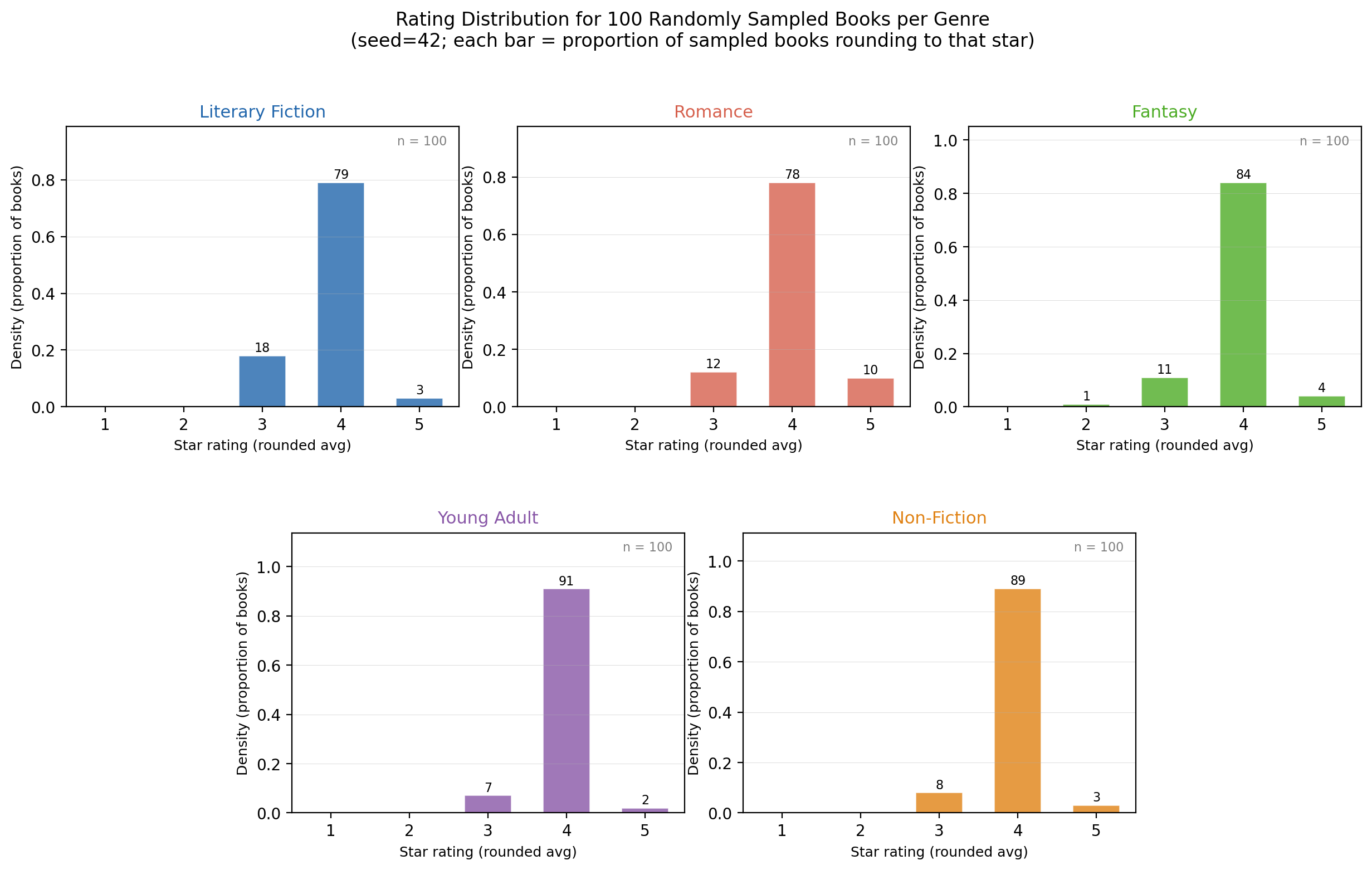
<p>My method of book choice makes crude approximations of $m_b$ and $\lvert\mathcal{K’}\rvert$, as determined by the book cover. To add some more information to my decision, I have recently begun to peruse Goodreads for their average rating. The average rating on a large enough sample marginally improves my estimate of $m_b$, but does nothing for my tastes (this is fine by me, because I like to be surprised). Unfortunately, this is what the Goodreads rating distribution looks like:</p>

<figure id="fig1">
  <img src="/assets/images/sample_ratings.png" alt="Goodreads rating distribution across genres, 2010–2017" />
  <figcaption>Figure 1. Data from <a href="https://cseweb.ucsd.edu/~jmcauley/datasets/goodreads.html#datasets">cseweb.ucsd.edu/~jmcauley/datasets/goodreads.html</a>, 2010–2017.</figcaption>
</figure>

<p>Now it’s entirely possible that the modal rating is a good decision rule — if the book scores $\geq 4$ stars, I should just buy it, but I’m a little skeptical about the modal rating being so high. This post will primarily focus on determining $m_b$ using Goodreads ratings. For a minute though, let’s consider the taste parameter, which I could solve for by reading users’ text reviews. This is still pretty noisy, because (a) the likelihood that I stumble across a user with my $\mathcal{K}$ (or a large subset of it) is pretty low, (b) I simply do not have the time to comb through people’s reviews, and (c) spoilers.</p>

<p>A good alternative to reading text reviews is social media, which is a relatively low-cognitive-effort tool for optimising taste-based consumption. BookTok (the literary corner of TikTok) emerged in 2019, and it doesn’t take a genius to know that popular content is taste-making. BookTok features creators who review books, providing detailed information on the content, theme, and genre (topped off with their personal experience). Popular videos have likes, reposts, and shares, which is a form of reviewing the review itself. If we assume that knowledge of the book’s true quality is increasing in the number of reviews ($n$) (and reviews of reviews), then TikTok is an excellent resource to maximise $\mathbf{E}[U_b]$.</p>

<p><em>Aside:</em> It also leads to taste convergence. Creators review more of the same books, creating a commercial feedback loop of epic proportions. Everyone is reading and talking about the same books, their adaptations, and their not-so-creative boilerplate bubble-font cartoon covers.</p>

<p>The advantage of consuming books that are “reviewed” $n$ times is massive — content has tags that let you filter for themes you enjoy, likes and comments provide enough information to predict with near certainty your utility from consuming the book. The rational agent always consumes the product with the highest expected utility.</p>

<p><em>Aside:</em> If you heavily use and rely on BookTok (or any content-creator based book-review system), then you can achieve $\mathbf{E}[U_b] = U_b$ by searching for a creator that has the same $\mathcal{K}$ as you. The original utility maximisation problem requires you to re-compute expected utility for <em>each book</em> you pick up. Choosing a creator with the same set of preferences as you eliminates this cognitive effort (assuming both your and the creator’s set of preferences stay fixed).</p>

<p>This is bad news for me. I don’t consume the content about books, and have already ironed my priors into a Hemingway-circlejerk shape, so the only review I do occasionally lean on is an average Goodreads rating. Why? If it’s above <span class="tex2jax_ignore">$20</span> (thank you, Canadian Publishing), and I have never read anything by the author, I appreciate some wisdom from the crowd. I suspect that at this point, the cost of curating a literary algorithm on any social media will require considerable interaction that I don’t want to partake in. Which leaves me archaically stranded on the now Amazon-owned-and-unchanged-since-2012 website.</p>

<p>This is incredibly unhelpful, because 5-star rating systems are right-skewed. Curating an algorithm that gives me detailed reviews imposes a higher cost than reading the raw rating averages on Goodreads and making a buy-or-not decision. It’s similar to the tradeoff problem that platforms face while designing a review system — they can elicit many coarse responses, or fewer detailed responses. Reducing the number or complexity of questions that a reviewer must answer increases the likelihood that she will complete the review (<a href="https://www.researchgate.net/publication/255686355_The_Long_and_Short_of_It_When_Does_Questinnaire_Length_Affect_Response_Rate">Bean and Roszkowski 1995</a>) at the cost of the information contained in each review. For me, this means that I could either get the average of a large number of coarse reviews instantly, or spend more time listening to one long and detailed review.</p>

<p>So I want to continue to use my Goodreads “look at the average” system, but with some confidence. To do this, I’ll take Murphy’s paper to Goodreads data and compute the optimal rating threshold that determines which books are worth my time.</p>

<h2 id="the-model">The Model</h2>

<p>Assume that the optimal review system is binary, and I want to determine some threshold value $k$ such that all books rated $k’$, for $k \leq k’$, are good, and I should buy them. For simplicity, I’ll stick to the paper’s language and motivate the review threshold decision for the platform, but it doesn’t change the spirit of this exercise.</p>

<p>Goodreads wants to design a review system that allows it to determine the unknown quality of a book. The platform chooses a review system (1–5 stars), and reviewers use their private signals and benefits to submit a review (private benefit from submitting a review, net of cost). The platform observes the set of submitted reviews, and then chooses to update its belief on the quality of the book.</p>

<p>A key assumption of this model is that the probability a reviewer submits a review is independent of a reviewer’s signal realisation. This is unrealistic: in practice reviewers with more extreme signals are more likely to submit reviews (<a href="https://doi.org/10.1016/j.geb.2014.01.007">Lafky 2014</a>; <a href="https://doi.org/10.25300/MISQ/2017/41.2.06">Hu, Pavlou, and Zhang 2017</a>). Common review systems, like 5-star reviews, are difficult to fine-tune because of reviewers’ extensive experience with similar systems: reviewers are likely to default to their own, private, thresholds (<a href="https://doi.org/10.1038/s41586-025-08599-7">Botelho et al. 2025</a>). Which is precisely why we’ll try to motivate a binary system, by solving for a threshold.</p>

<p><em>Note:</em> We’ll hand wave over quite a bit of theory, but the key insight here is that the symmetric binary review system is the optimal binary review system if and only if reviewers are sufficiently heterogeneous.</p>

<h2 id="data-and-heterogeneity">Data and Heterogeneity</h2>

<p>We’ll use the same data used to plot <a href="#fig1">Figure 1</a>, and take the model to it. I take the top 1,000 books per genre, from 2010–2017, and use exact per-book star-count histograms from the raw reviews file (individual star ratings 1–5).<br />
<strong>Sample Selection:</strong> Choosing the top 1,000 books is a necessary evil (although I could sample more). Think of it as imposing a lower bound for $m_b$ on all books.</p>

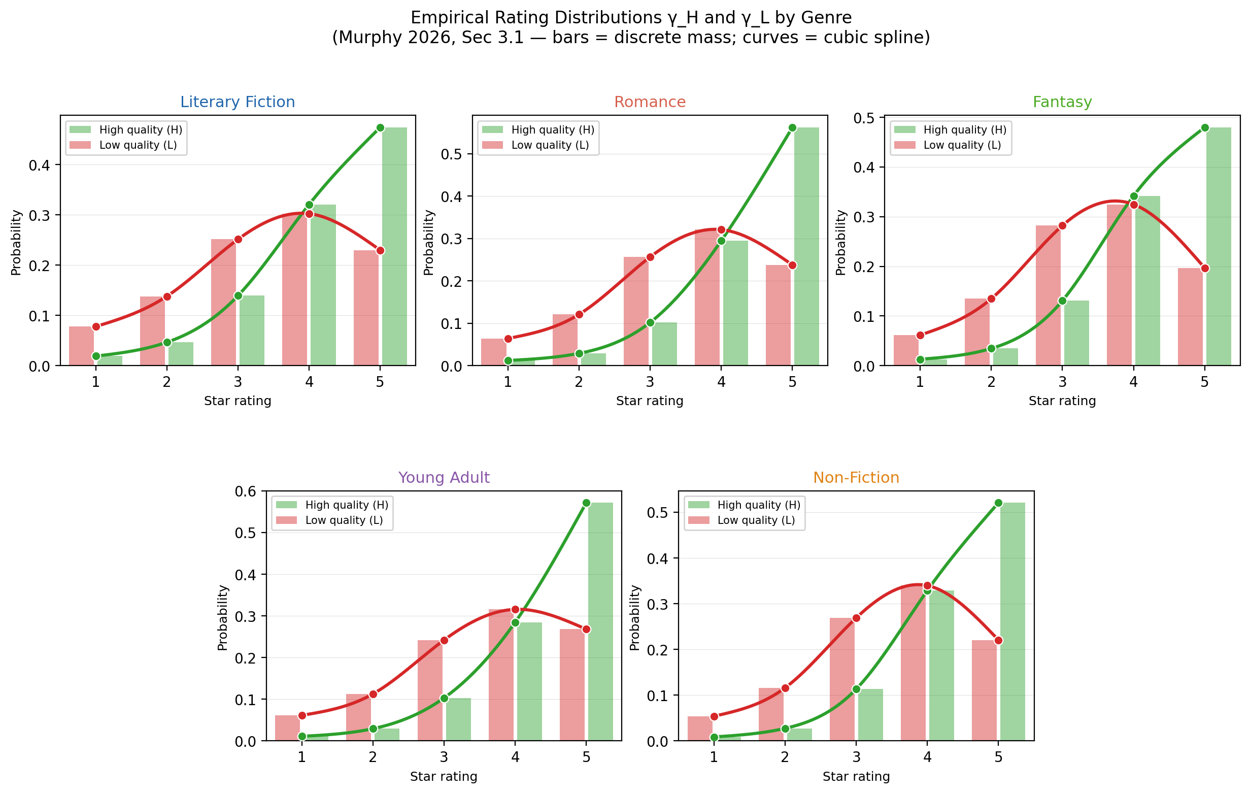
<p>First, we want to determine Goodreads’ learning rate and heterogeniety: given its 5-star review system, how many reviews does it take for the platform to learn a book’s true quality? Let $\gamma_H$ and $\gamma_L$ be the distributions of reviewer signals conditional on each quality state (High or Low). This allows us to determine heterogeneity. If $\gamma_H$ and $\gamma_L$ barely overlap, a single review gives the platform a lot of information. If they overlap heavily, each review is noisy and the platform needs many more reviews to learn the state. This makes intuitive sense — if signals are extreme, we need few of them to learn the state.</p>

<p>In the figure below, each of the five panels corresponds to one genre. Within each panel there are two sets of five side-by-side bars — one set for H (high-quality) books and one for L (low-quality) books — showing the empirical probability mass at each star value 1 through 5:</p>

<ul>
  <li><strong>Green bars — “High quality” books (H):</strong> the top third of books in the genre, ranked by their average rating across all reviews. For each book we count the raw number of 1-star, 2-star, …, 5-star reviews it received; the bars show the pooled share across all H books in the genre.</li>
  <li><strong>Red bars — “Low quality” books (L):</strong> the bottom third of books by the same ranking. The middle third is discarded to sharpen the contrast between quality states.</li>
</ul>

<p>The y-axis is the share of reviews in each star bucket (sums to 1 within each quality group).</p>

<figure id="fig2">
  <img src="/assets/images/01_rating_distributions_smoothed.png" alt="Empirical rating distributions γ_H and γ_L by genre" />
  <figcaption>Figure 2. Empirical rating distributions $\gamma_H$ and $\gamma_L$ by genre (bars = discrete probability mass; curves = cubic spline).</figcaption>
</figure>

<p>This is a more informative picture of how user signals are distributed on the platform:</p>

<ul>
  <li>In all genres, H books are concentrated at 4–5 stars (75–87% of H reviews), while L books are more spread (45–55% of L reviews reach 4–5 stars). The 2–3 star region in particular is much denser for L than H. <em>We look at the overlap between H and L splines. The splines diverge at 4 for all genres, which means that 4–5 star books are consistently good picks for me. Put differently, signals $\leq 4$ don’t allow me to confidently distinguish H and L books, and are thus not credible. This matches what we learnt from the <a href="#fig1">Figure 1</a> rating distribution, which says that books rated $\geq 4$ are good choices.</em></li>
  <li>Young Adult H books have the most extreme 5-star concentration: 57.2% of all H reviews give 5 stars. Non-Fiction and Romance H also exceed 50% at 5 stars. Literary Fiction H is the least concentrated at 5 (47.4%) and has more mass at 3–4 stars. <em>Young Adult, Non-Fiction, and Romance readers dispense 5-star ratings fairly frequently, which throws a wrench in the $\geq 4$ decision rule. The overall right skew in platform ratings is driven by these genres. Why is this a problem if we expect H books to be better anyway? Ideally, you want the distribution of ratings to be flat (or flat-ish), so that each rating threshold captures meaningful information — in other words, you want tastes to be sufficiently heterogeneous on a 5-star rating system.</em></li>
  <li>Note that Literary Fiction (which is the genre I happen to care most about) has the most uniform spread across all five stars (8%/14%/25%/30%/23%), resembling an almost flat distribution. <em>The lit-fic distribution is encouraging. If each threshold captures meaningful information, then tastes are sufficiently heterogeneous and we should be able to determine a decision threshold based on averages alone. Things look a little bleak for other genres, where the skew indicates that we might want to pay more attention to the distribution of reviews than the average alone.</em></li>
</ul>

<h2 id="optimal-thresholds">Optimal Thresholds</h2>

<p>Now that we have a learning rate and have established that the data (for literary fiction) is sufficiently heterogeneous, we want to determine the binary cutoff threshold that will let us pick a good book, solely based on its average rating. If Goodreads replaced its 5-star system with a binary (thumbs-up / thumbs-down) system, what single cutoff point maximises the information the platform retains about book quality?</p>

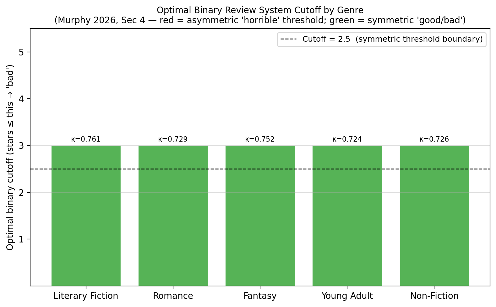
<p>Each bar represents one genre. The bar height is the optimal cutoff star value: a cutoff of 3 means “rate 3 stars or below = thumbs down; 4 stars or above = thumbs up.” <em>The region $3 &lt; x &lt; 4$ is the ambiguous middle. We can’t say with confidence if these books are good or bad.</em></p>

<p>The dashed horizontal line at 2.5 is the boundary between symmetric and asymmetric thresholds. Bars above 2.5 (green) represent symmetric or “good/bad” thresholds — the platform is asking “did you like it?” Bars below 2.5 (red, none here) would represent asymmetric “horrible” thresholds (the platform would be asking “was this terrible?” rather than “was this good?”)</p>

<p><strong>Why?</strong> When reviewers are heterogeneous, a 1-star review might just mean a mismatch in taste, so the platform gets more information by asking the symmetric question (“did you like it?”) and drawing the line at the midpoint of the signal space.</p>

<p>The $\kappa$ value annotated above each bar is the relative information: the fraction of the full 5-star system’s learning efficiency that the optimal binary system retains.</p>

<p><em>Aside:</em> By Theorem 1 of <a href="https://mjhmurphy.github.io/files/pdf/ClicksComments_mjHM.pdf">Murphy (2026)</a>, a binary system is preferred to the 5-star system when binary reviews are submitted at least $1/\kappa$ times as often. The breakeven multipliers are greater than 1 (Literary Fiction: 1.31×; Romance/Non-Fiction/Young Adult: ~1.37–1.38×), which means that we need more reviews for the binary system to be judged against exact star-counts. I’m choosing to ignore this for now.</p>

<figure id="fig3">
  <img src="/assets/images/04_optimal_thresholds.png" alt="Optimal binary threshold cutoff by genre, annotated with κ values" />
  <figcaption>Figure 3. Optimal binary cutoff threshold by genre. Bar colour indicates symmetric (green) vs asymmetric (red) threshold. $\kappa$ values annotated above each bar.</figcaption>
</figure>

<p>Every genre’s optimal binary system maps 1–3 stars to “bad” and 4–5 stars to “good.” This is the symmetric threshold, coded green. It is consistent with Murphy’s prediction for the heterogeneous-reviewer regime. <em>Note the $\kappa$ value: the penalty of compressing to binary is large — I’m losing over 20% of useful information when I compress my ratings. However, the information loss is the least in literary fiction, because tastes are sufficiently heterogeneous.</em></p>

<figure id="fig4">
  <img src="/assets/images/05_binary_landscape.png" alt="Full κ landscape across all binary threshold cutoffs and genres" />
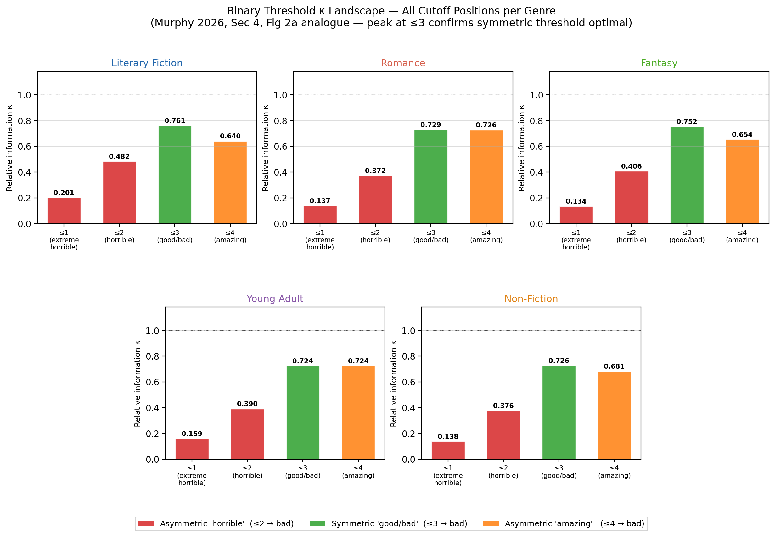
  <figcaption>Figure 4. Full empirical $\kappa$ landscape across all binary cutoff thresholds and genres.</figcaption>
</figure>

<p>This figure reveals the full empirical $\kappa$ landscape, showing which regime Goodreads occupies and how steep the information penalty is for moving away from the optimum.</p>

<p><em>For Romance, Young Adult, and (to a lesser extent) Non-Fiction — the symmetric and asymmetric thresholds for good and amazing books are the same. Put differently, on a 5-star scale, the fourth and fifth stars are functionally equivalent to three stars. This makes an optimal decision threshold of 3 iffy, because we have no credible way to differentiate the good from the excellent. In an ideal world, I should be able to differentiate a good romance novel (say, Book Lovers) from an excellent romance novel (Oscar and Lucinda), but it doesn’t look like Goodreads is the ideal setting for that.</em></p>

<p>In any case, I would like to minimise the possibility of a bad reading experience. For these genres, I will only choose books rated $\geq 4$, since they will be <strong>at least</strong> good, and possibly amazing (although I will not be able to differentiate this ex-ante).<sup id="fnref:1" role="doc-noteref"><a href="#fn:1" class="footnote" rel="footnote">1</a></sup></p>

<p>Now let’s go back to literary fiction (and fantasy), where good-or-not (symmetric) and amazing-or-horrible (asymmetric) thresholds capture different information. This is excellent news for me, because it means that a threshold rating of $\geq 3$ is a sufficient statistic for me to determine that a book will be <strong>at least</strong> good, and a rating of $\geq 4$ means that a book will be great. My problem is now solved.<sup id="fnref:2" role="doc-noteref"><a href="#fn:2" class="footnote" rel="footnote">2</a></sup></p>

<hr />

<div class="footnotes" role="doc-endnotes">
  <ol>
    <li id="fn:1" role="doc-endnote">
      <p>In an ideal world, Goodreads will redesign its rating system for these genres to an asymmetric binary. <a href="#fnref:1" class="reversefootnote" role="doc-backlink">&#8617;</a></p>
    </li>
    <li id="fn:2" role="doc-endnote">
      <p>In practice, I’m not always drawing from the top 1,000 books in a genre, so the rating threshold helps me solve for $m_b$ each time. Determining whether $b$ satisfies my idiosyncratic tastes is still my cross to bear. <a href="#fnref:2" class="reversefootnote" role="doc-backlink">&#8617;</a></p>
    </li>
  </ol>
</div>]]></content><author><name></name></author><summary type="html"><![CDATA[This week at the CETC, I attended M. Murphy’s talk on optimal review design. This post leans on his paper, “Clicks or Comments? The quality-quantity trade-off of review systems”, to solve a very pedantic problem. It was written across conference sessions, so errors are both highly likely and entirely my own.]]></summary></entry><entry><title type="html">My TODO List</title><link href="https://vaze-esha.github.io/2026/05/01/todo-list.html" rel="alternate" type="text/html" title="My TODO List" /><published>2026-05-01T00:00:00+00:00</published><updated>2026-05-01T00:00:00+00:00</updated><id>https://vaze-esha.github.io/2026/05/01/todo-list</id><content type="html" xml:base="https://vaze-esha.github.io/2026/05/01/todo-list.html"><![CDATA[<p>Instead of using a notebook (or three crumpled receipts), I’ve moved to a TODO setup that lives in my shell config file.</p>

<hr />

<ol>
  <li>Paste the following block in your shell config file:</li>
</ol>

<div class="language-bash highlighter-rouge"><div class="highlight"><pre class="highlight"><code><span class="c"># TODO SCRIPT. use as move_todo line_number</span>
move_todo<span class="o">()</span> <span class="o">{</span>
    <span class="nb">local </span><span class="nv">linenum</span><span class="o">=</span><span class="nv">$1</span>
    <span class="nb">local </span><span class="nv">date_today</span><span class="o">=</span><span class="si">$(</span><span class="nb">date</span> +<span class="s2">"%d/%m"</span><span class="si">)</span>
    <span class="nb">local </span><span class="nv">time_now</span><span class="o">=</span><span class="si">$(</span><span class="nb">date</span> +<span class="s2">"%H%M"</span><span class="si">)</span>

    <span class="c"># Add date header if not already present</span>
    <span class="k">if</span> <span class="o">!</span> <span class="nb">grep</span> <span class="nt">-q</span> <span class="s2">"^</span><span class="nv">$date_today</span><span class="s2">"</span> <span class="k">done</span><span class="p">;</span> <span class="k">then
        </span><span class="nb">echo</span> <span class="s2">"</span><span class="nv">$date_today</span><span class="s2">"</span> <span class="o">&gt;&gt;</span> <span class="k">done
    fi</span>

    <span class="c"># Move line with timestamp and checkbox</span>
    <span class="nb">sed</span> <span class="nt">-n</span> <span class="s2">"</span><span class="k">${</span><span class="nv">linenum</span><span class="k">}</span><span class="s2">p"</span> todo <span class="se">\</span>
        | <span class="nb">sed</span> <span class="s2">"s/^</span><span class="se">\[\]</span><span class="s2">/[X] </span><span class="k">${</span><span class="nv">time_now</span><span class="k">}</span><span class="s2">:/"</span> <span class="o">&gt;&gt;</span> <span class="k">done</span>

    <span class="c"># Delete the original line from todo</span>
    <span class="nb">sed</span> <span class="nt">-i</span> <span class="s1">''</span> <span class="s2">"</span><span class="k">${</span><span class="nv">linenum</span><span class="k">}</span><span class="s2">d"</span> todo
<span class="o">}</span>
</code></pre></div></div>

<ol>
  <li>
    <p>Make a <code class="language-plaintext highlighter-rouge">todo</code> file and a <code class="language-plaintext highlighter-rouge">done</code> file.</p>
  </li>
  <li>
    <p>Add an item to your <code class="language-plaintext highlighter-rouge">todo</code> list. Some examples:</p>
  </li>
</ol>

<div class="language-plaintext highlighter-rouge"><div class="highlight"><pre class="highlight"><code>[] post TODO script
[] drink coffee
</code></pre></div></div>

<ol>
  <li>To move an item to the <code class="language-plaintext highlighter-rouge">done</code> list:</li>
</ol>

<div class="language-plaintext highlighter-rouge"><div class="highlight"><pre class="highlight"><code>move_todo 1
</code></pre></div></div>

<ol>
  <li>The <code class="language-plaintext highlighter-rouge">done</code> file is now updated:</li>
</ol>

<div class="language-plaintext highlighter-rouge"><div class="highlight"><pre class="highlight"><code>[X] 0756: post TODO script
</code></pre></div></div>

<ol>
  <li>Make sure to change into the directory where your <code class="language-plaintext highlighter-rouge">done</code> and <code class="language-plaintext highlighter-rouge">todo</code> files live before using <code class="language-plaintext highlighter-rouge">move_todo</code>.</li>
</ol>]]></content><author><name></name></author><summary type="html"><![CDATA[Instead of using a notebook (or three crumpled receipts), I’ve moved to a TODO setup that lives in my shell config file.]]></summary></entry><entry><title type="html">Vancouver Café Rankings</title><link href="https://vaze-esha.github.io/2026/05/01/vancouver-cafe-rankings.html" rel="alternate" type="text/html" title="Vancouver Café Rankings" /><published>2026-05-01T00:00:00+00:00</published><updated>2026-05-01T00:00:00+00:00</updated><id>https://vaze-esha.github.io/2026/05/01/vancouver-cafe-rankings</id><content type="html" xml:base="https://vaze-esha.github.io/2026/05/01/vancouver-cafe-rankings.html"><![CDATA[<p>This is <strong>not</strong> a definitive coffee-snob approved ranking. Unfortunately, despite going to upwards of three coffee shops a week (on average), I’m the most satisfied by a bottomless, biting-strong drip than by any other type of coffee. Fortunately, I do like working in cafés, and thus have a large <em>n</em> inference on what “good coffee” tastes like.</p>

<p>Since I like consuming jitter-inducing amounts of caffeine before I noisily type on my computer, and I don’t like search costs, here is a list of Vancouver cafés to work at, that have:</p>

<p>(a) good coffee<br />
(b) outlets<br />
(c) nice tables <sup id="fnref:1" role="doc-noteref"><a href="#fn:1" class="footnote" rel="footnote">1</a></sup><br />
(d) good music on the speakers (not too loud) <sup id="fnref:2" role="doc-noteref"><a href="#fn:2" class="footnote" rel="footnote">2</a></sup><br />
(e) wi-fi</p>

<p>Every shop listed here satisfies (a)–(e), with idiosyncratic pros and cons. Admittedly, this list is incomplete.</p>

<hr />

<p><strong>1. <a href="https://www.moduscoffee.com/">Coffee Roastery Modus</a></strong><br />
This is my favourite coffee shop in town. Incredible coffee and pastries, and the baristas play fantastic music (possibly a Mount Pleasant fixed effect). They’re pretty small but never very busy, and get bonus points for nice bay windows. On the weekends there’s local roastery/pastry pop-ups which have (so far), never let me down.</p>

<p><strong>2. <a href="https://www.arbutuscoffee.ca/">Arbutus Coffee House</a></strong><br />
Cozy, close second. Nice sandwiches and iced drinks. Primarily plays the MJ Lenderman variety of y’allternative music (complimentary). Very cozy, great furniture and decor. Decently busy in the mornings and on weekends. Looks out on a beautiful bike-lane tree-lined intersection.</p>

<p><strong>3. <a href="https://www.fogliftercoffee.com/">Foglifter Coffee Roasters</a></strong><br />
High exposed ceilings, tastefully decorated. A wide selection of beautifully done baked goods and seasonal drinks, and the coffee is always great. Well lit with all-round windows, and every table has an outlet. Unfortunately, the music quality in this place is very variable. The rest of its qualities make up for this (otherwise glaring) deficiency. No wi-fi on weekends.</p>

<p><strong>4. <a href="https://www.luminecoffee.com/">Lumine Coffee</a></strong><br />
$8 espresso flight. Small selection of baked goods, the croissants are really nice. Seating in the back of the shop is great, front of house is a tad bit too small. Once again, $8 espresso flight.</p>

<p><strong>5. <a href="https://www.analogcoffee.ca/">Analog Coffee</a></strong><br />
Despite my personal beef with the chain for being mean to my roommate (their former employee), this is a solid place to work. It’s often dominated by people with laptops for this reason. The coffee is uniformly good and all their locations have a lot of seating. I like the Yaletown location the most. No wi-fi on weekends.</p>

<p><strong>6. <a href="https://www.aperturecoffeebar.com/">Aperture Coffee Bar</a></strong><br />
Lots of seating, very cozy (especially in the winter). Open late, has great wi-fi, jazz music, and sandwiches. Serves alcohol at night. I’ve spent a lot of hours here in the last 5 years and they’ve all been good.</p>

<p><strong>7. <a href="https://www.kafkascoffee.ca/">Kafka’s Coffee Roasting and Bakery</a></strong><br />
Massive. Large windows, very high ceilings, attached to the art school. The coffee is good, and they have a nice selection of sandwiches on house-baked sourdough bread. Very quiet in the summer, with good air conditioning.</p>

<p><strong>8. <a href="https://funk.coffee/">FUNK. Coffee Bar</a></strong><br />
Big windows and lots of seating. Good music (as reported by David, unverified by me). I like the coffee here, and there’s occasional pop-ups for a variety of merchandise. Unrelated to working there, their branding is pretty fun.</p>

<hr />

<p>Now, here is a list of cafés with good coffee (and in some cases, baked goods), that you cannot work at. Maybe take a book or a friend.</p>

<ol>
  <li>Peace and Culture Coffee</li>
  <li>Yuán Coffee</li>
  <li>Toña Bakery and Café</li>
  <li><a href="https://birdsandbeets.ca/">Birds and the Beets</a></li>
  <li><a href="https://oideoide.com/">Oidé Coffee</a></li>
  <li><a href="https://tvdinnershop.ca/">TV Dinner Market and Café</a></li>
  <li><a href="https://federalstore.ca/">The Federal Store Luncheonette and Grocer</a></li>
  <li><a href="https://platform7coffee.com/">Platform 7 Coffee</a></li>
</ol>

<hr />

<div class="footnotes" role="doc-endnotes">
  <ol>
    <li id="fn:1" role="doc-endnote">
      <p>I suffer from the wobbly-table curse. On any given day, the table I choose will be rocky at best. This actually makes my claim to (c) stronger because I persevere despite the horrors, managing to stay relatively unbiased despite my poor luck. <a href="#fnref:1" class="reversefootnote" role="doc-backlink">&#8617;</a></p>
    </li>
    <li id="fn:2" role="doc-endnote">
      <p>I strongly believe that there is an objective threshold for good music before subjective taste-based preferences kick in. <a href="#fnref:2" class="reversefootnote" role="doc-backlink">&#8617;</a></p>
    </li>
  </ol>
</div>]]></content><author><name></name></author><summary type="html"><![CDATA[This is not a definitive coffee-snob approved ranking. Unfortunately, despite going to upwards of three coffee shops a week (on average), I’m the most satisfied by a bottomless, biting-strong drip than by any other type of coffee. Fortunately, I do like working in cafés, and thus have a large n inference on what “good coffee” tastes like.]]></summary></entry><entry><title type="html">Notes for Data Analysis</title><link href="https://vaze-esha.github.io/2025/03/01/notes-for-data-analysis.html" rel="alternate" type="text/html" title="Notes for Data Analysis" /><published>2025-03-01T00:00:00+00:00</published><updated>2025-03-01T00:00:00+00:00</updated><id>https://vaze-esha.github.io/2025/03/01/notes-for-data-analysis</id><content type="html" xml:base="https://vaze-esha.github.io/2025/03/01/notes-for-data-analysis.html"><![CDATA[<h2 id="introduction">Introduction</h2>

<p>Last term, I collected every question that my classmates asked me (as they worked on their theses), and compiled notes to make a little guide that could (potentially) be useful for someone working with economic data for the first time. The primary purpose of this document is to give you some guidance on how to organize your project and manage your do-files in a way that is reproducible and clean.</p>

<p>I’ll go through some basic do-file structuring practices to make your workflow easier to follow if this is your first time touching a large-ish project in Stata. Even if you feel that replication is not paramount for an undergraduate project (and perhaps it isn’t), it’s still useful to organize your data with that goal in mind, both for your own convenience and for that of your readers’.</p>

<p>I wrote this guide because most undergraduates who don’t work as RAs haven’t had the pleasure of reading <a href="https://web.stanford.edu/~gentzkow/research/CodeAndData.xhtml">Code and Data for the Social Sciences: A Practitioner’s Guide</a>, and besides, the scale of most undergraduate projects is smaller and the scope much narrower. This guide caters to that small corner of writing code for economics, and is easier to follow (especially if you’re not in the business of writing shell scripts for automation) because it only assumes a basic working knowledge of Stata.</p>

<hr />

<p><em>Note:</em> There is no dearth of resources that are specifically geared towards writing code for the social sciences (see <a href="https://github.com/jdingel/projecttemplate">here</a>, <a href="http://plain-text.co/">here</a>, and also <a href="https://www.youtube.com/watch?v=ZSunU9GQdcI">here</a>). This guide is not an attempt to reinvent that (nearly) perfect wheel. I wrote this because many people I know found existing resources to be too broad in scope to serve as a meaningful reference for their 2-term projects. All the resources above (and some more at the end of this document) are excellent for those truly wrestling with big data and teams. However, if you’re trying to get through a thesis class (or just doing a small project to satisfy your curiosity), then I suspect this guide will be of some use to you.</p>

<hr />

<p>Why is this guide focused on Stata? The target audience for this guide is an economics undergraduate writing their first paper/project, and it is highly likely that they will use Stata (easy, caters to economics, recommended by instructors).<sup id="fnref:1" role="doc-noteref"><a href="#fn:1" class="footnote" rel="footnote">1</a></sup></p>

<hr />

<p><em>Side-note:</em> Stata is weird, and has an overly specific use case (academic economics). The error messages are largely useless, the documentation is lean, the online forums are a scary place (I’m looking at you, Statalist), and most LLM chatbots perform unsatisfactorily when asked to write Stata code (clunky, inefficient, and ugly to look at). I’m not sure what the future looks like for Stata, but it’s been here long enough, and for all my complaining it is very convenient for the niche it serves. That said, I don’t think I would bother touching it if I wasn’t enrolled in an economics degree.</p>

<hr />

<p>My main purpose here is to introduce a replicable format of code and data organization for smaller projects, the knowledge for which is primarily borrowed from my time as a research assistant, spent working on replication packets for papers. Per usual, all errors are my own.</p>

<p>To make this easy to follow, I describe a hypothetical project, and then show you how I would organize it. I try to keep this guide as linear as possible, although that is very rarely the case when you actually start getting your hands dirty.</p>

<h2 id="data-organization">Data Organization</h2>

<p><strong>Hypothetical project</strong>: We’re trying to measure the impact of an employment guarantee program on female unemployment rates in the Canadian province of Newfoundland. Assume that we live in a perfect world where the program assignment was randomized, and the government gives us a full dataset of treated and control populations with their demographic details. To help our analysis, we download a zip-code level map of Newfoundland, and a dataset containing household income, number of children and the addresses of everyone enrolled in the program.</p>

<p>These datasets constitute our “raw inputs”. We will create a project directory on Dropbox (or any other file-hosting service that you prefer) where all our data will live.<sup id="fnref:2" role="doc-noteref"><a href="#fn:2" class="footnote" rel="footnote">2</a></sup></p>

<p>Here’s what a typical data directory would look like:</p>

<div class="language-plaintext highlighter-rouge"><div class="highlight"><pre class="highlight"><code>project_newfoundland_data       # main data directory
├── 0_raw_input                 # raw data directory
│   ├── 0_1_rct.xlsx
│   ├── 0_2_zip_codes.shp
│   └── 0_3_income_and_covariates.xlsx
├── 1_intermediate              # processed data directory
│   ├── 1_1_rct_cleaned.dta
│   ├── 1_2_zip_codes_rct_merged.dta
│   └── 1_3_covariates_rct_merged.dta
└── 2_final                     # datasets used for final analysis
   └── 2_1_rct_analysis.dta    # contains variables for analysis
                               # folder typically contains final datasets used for regressions, tables and figures
</code></pre></div></div>

<p>Sub-directory <code class="language-plaintext highlighter-rouge">1_intermediate</code> contains data that has been cleaned (drop duplicate observations, harmonize variables, address consistency issues) and <code class="language-plaintext highlighter-rouge">2_final</code> contains the processed datasets for your final analysis. When you upload your replication packet, the only datasets that you (ideally) include in it are your raw inputs, and let your code generate the rest.</p>

<p>This makes your data organization easy to follow for someone who has limited context about the project, while also making it convenient for your future self to follow your data cleaning methodology.<sup id="fnref:3" role="doc-noteref"><a href="#fn:3" class="footnote" rel="footnote">3</a></sup></p>

<hr />

<p><em>Aside:</em> Even when you first start, organize your project with a replication package in mind. Which means two things:</p>

<ol>
  <li>A complete stranger, given reasonable instructions, should be able to replicate every result in your project by running your code locally.</li>
  <li>Said stranger (assuming that they have non-zero Stata knowledge) should understand your code, or at the very least be able to parse the rudiments of your data analysis.</li>
</ol>

<p>Why should you care? First, if there are some glaring econometric issues with how you analyze your data, well documented and replicable files will help someone point them out (and save you tons of trouble). Second, future you is effectively a complete stranger (you will forget why you used that specific transformation two summers ago). Third, it’s good for accountability: you should care about doing research that is transparent and replicable. Think of it as creating a public good.</p>

<h2 id="code-organization">Code Organization</h2>

<p>The way you organize your code mimics the data storage structure. I recommend creating a repository on GitHub with relevant sub-directories to store all your code.<sup id="fnref:4" role="doc-noteref"><a href="#fn:4" class="footnote" rel="footnote">4</a></sup></p>

<div class="language-plaintext highlighter-rouge"><div class="highlight"><pre class="highlight"><code>project_newfoundland_do  # main code directory
├── setup.do   
├── master.do
├── 0_import_and_process       # import and process data
│   ├── 0_1_rct_import.do
│   ├── 0_2_zip_codes_import.do
│   └── 0_3_income_and_covariates_import.do
├── 1_intermediate             # processed data directory
│   ├── 1_1_rct_cleaning.do
│   ├── 1_2_create_dataset.do
│   └── 1_3_covariates_rct_create_dataset.do  # create your datasets
│                                             # files here correspond (see numbering) to datasets that they produce as outputs
│                                             # this keeps things easy to keep track of
└── 2_final                    # datasets used for final analysis
   ├── 2_1_rct_analysis.do    # your main analysis file
   └── 2_2_figures_maps.do    # some figures for your paper
</code></pre></div></div>

<hr />

<p>So what are <code class="language-plaintext highlighter-rouge">master.do</code> and <code class="language-plaintext highlighter-rouge">setup.do</code>? You want a stranger to be able to replicate this code by running a single file (literally at the push of a button), and a master do-file lets you do that. Now that all your data and code is stored based on its use-case, here are two files you should consider adding to make this workflow easier to run:<sup id="fnref:5" role="doc-noteref"><a href="#fn:5" class="footnote" rel="footnote">5</a></sup></p>

<h2 id="setupdo"><code class="language-plaintext highlighter-rouge">setup.do</code></h2>

<p>More often than not, people do the following:</p>

<div class="language-plaintext highlighter-rouge"><div class="highlight"><pre class="highlight"><code>use "/User/john_doe/Dropbox/project_newfoundland_data/0_raw_input/0_1_rct.xlsx"
…
use "/User/john_doe/Dropbox/project_newfoundland_data/1_intermediate/1_1_rct_cleaned.dta"
…
use "/User/john_doe/Dropbox/project_newfoundland_data/2_final/2_1_rct_analysis.dta"
</code></pre></div></div>

<p>And on and on. You get the idea. While there’s nothing wrong with it (your code will run), the repetition alone should ring some alarm bells. Surely there must be a way to make this less clunky (there is). <strong>Here’s what you can do</strong>: create a do-file that lives in your main code repository and dump all your directory paths into it. Ideally, you want to be able to use this file across multiple sub-directories for your project, so the paths you use are “global” macros (read up on local and global scope in Stata to better understand what you need)</p>

<div class="language-plaintext highlighter-rouge"><div class="highlight"><pre class="highlight"><code>global $workingdir "/User/john_doe/Dropbox/project_newfoundland_data"
global $raw_input_dir "$workingdir/0_raw_input"
global $intermediate_data_dir "$workingdir/1_intermediate_data"
…
</code></pre></div></div>

<p>Now you’re free to use:</p>

<div class="language-plaintext highlighter-rouge"><div class="highlight"><pre class="highlight"><code>use "$raw_input_dir/0_1_rct.xlsx"
</code></pre></div></div>

<p>Which saves some space, looks better, and is much more convenient than printing the whole file path over and over. For a typical project, I would create a setup file that sets all my global data directories, installs any package dependencies, sets any locals that I need, and so on.</p>

<h2 id="masterdo"><code class="language-plaintext highlighter-rouge">master.do</code></h2>

<p>A master do-file sequentially calls every do-file in your project. When you’re working with larger projects, they’re convenient because they save you the trouble of having to individually run files. Coming back to replication, when you finally make your project publicly available your master file lets people run your code at the click of a button instead of having to figure out the right order needed to generate your results. It looks something like this:</p>

<div class="language-plaintext highlighter-rouge"><div class="highlight"><pre class="highlight"><code>global $dodir "User/john_doe/project_newfoundland_do" # point to wherever John cloned his repository, add to setup file
…
do "$dodir/2_analysis/2_1_rct_analysis.do"
do "$dodir/2_analysis/2_2_figures_maps.do"
...
</code></pre></div></div>

<p>Some people also like having their paths in the master file instead of in <code class="language-plaintext highlighter-rouge">setup.do</code> – it’s really up to you, and both of these steps are technically optional, but they make life easier and your code more legible in the long and short run. If you want even more control, you can make a master file for each code sub-directory to run each section of your data cleaning and analysis separately.</p>

<p>Great. Now you have neatly organized boxes, and specific uses for them all. Write down exactly what’s in each file, each directory, each sub-directory (Make a README file, make two, make four). Be as detailed as possible, and then cut the fluff later when you feel like you have a better handle on how everything works.</p>

<p>When making your do-files, write comments. Be verbose. Try to make everything as simple as possible, and then go back again and make it simpler. If you find yourself repeating the same line of code over and over, there’s a better way to do it. It always helps to imagine a complete stranger who knows nothing about your project, and then write your code so that given minimal context they’re able to make sense of what it does.<sup id="fnref:6" role="doc-noteref"><a href="#fn:6" class="footnote" rel="footnote">6</a></sup></p>

<hr />

<p><strong>Closing Notes:</strong>
A large part of this guide was born out of frustration from watching people clear-reload their datasets from the depths of their downloads folder every single time they ran a regression. I realized that it would be useful (not to my cohort, but perhaps future ones) to have a short text that tells you how to structure your project so that it’s easier for you, and whoever is helping you to understand it. This is, as stated previously, a very bare-bones guide and should work fine for a small to medium sized project. Eventually, you’ll want to learn how to automate more of your workflow — you can learn basic shell-scripting (here’s a fun <a href="https://tldp.org/LDP/abs/html/index.html">book</a>), or just use Python. As your projects get larger, you’ll even want to automate things like importing raw-inputs from a directory (it’s also fun, even when you don’t have to do it — I learnt how to use my computer pretty late in life, and I’m still fascinated by how cool and easy it is to automate really simple tasks).<sup id="fnref:7" role="doc-noteref"><a href="#fn:7" class="footnote" rel="footnote">7</a></sup> If you’re comfortable following a document less hand-holdy (and more general), then you should read <a href="https://web.stanford.edu/~gentzkow/research/CodeAndData.xhtml">Code and Data for the Social Sciences</a>.</p>

<p>Other fun resources you can look at (if you’re interested in the general concept of reproducible research):</p>

<ol>
  <li><a href="https://i4replication.org/about.html">Institute for Replication</a></li>
  <li>Browse AER papers’ replication packages (for inspiration)</li>
</ol>

<h2 id="further-reading">Further Reading</h2>

<p>Some additional resources I use and like</p>

<ol>
  <li><a href="https://ljristovska.com/assets/docs/coding_for_econs_20190221.pdf">Coding for Economists: A Language-Agnostic Guide to Programming for Economists</a></li>
  <li><a href="https://www.aeaweb.org/articles?id=10.1257/jep.28.1.209">An Economist’s Guide to Visualizing Data</a></li>
  <li><a href="https://pubs.aeaweb.org/doi/pdf/10.1257/jep.35.3.193">Evidence on Research Transparency in Economics</a></li>
  <li>Nick Hagerty has a cool course on <a href="https://github.com/msu-econ-data-analytics/course-materials#external-resources">advanced data analytics in R</a>, with a <a href="https://raw.githack.com/msu-econ-data-analytics/course-materials/main/data-cleaning-checklist/Data-Cleaning-Checklist.pdf">data cleaning checklist</a> that’s concise and useful.</li>
</ol>

<div class="footnotes" role="doc-endnotes">
  <ol>
    <li id="fn:1" role="doc-endnote">
      <p>You’re more than welcome to use it for organizing your code and analysis in any other language. This is not a “how to write code for (undergraduate) economic data analysis guide”, so the general principles extend to pretty much whatever language you choose to work in. <a href="#fnref:1" class="reversefootnote" role="doc-backlink">&#8617;</a></p>
    </li>
    <li id="fn:2" role="doc-endnote">
      <p>You can also do this locally, especially if you’re the only one working on the project. <a href="#fnref:2" class="reversefootnote" role="doc-backlink">&#8617;</a></p>
    </li>
    <li id="fn:3" role="doc-endnote">
      <p>Even if you’re like me and claim you have perfect memory, as your project gets larger and contains a mountain of data it’s better to have it corralled away into specific boxes than not. The added convenience comes from the fact that your code generates everything except the raw inputs, so you can make edits to your analysis more conveniently as time passes. <a href="#fnref:3" class="reversefootnote" role="doc-backlink">&#8617;</a></p>
    </li>
    <li id="fn:4" role="doc-endnote">
      <p>Even if you’re the only one working on the project, it’s incredibly useful to have a record of the changes you make. Version control will save you time and keep you accountable. If it makes life easier (and you don’t want to go through the mental gymnastics of learning command line functionality to use GitHub), consider getting GitHub Desktop to manage your do-files. <a href="#fnref:4" class="reversefootnote" role="doc-backlink">&#8617;</a></p>
    </li>
    <li id="fn:5" role="doc-endnote">
      <p>Sorry for flip-flopping between 0/1 indexing, but that’s just how I number these. You probably want to change that based on your philosophical and aesthetic bent. <a href="#fnref:5" class="reversefootnote" role="doc-backlink">&#8617;</a></p>
    </li>
    <li id="fn:6" role="doc-endnote">
      <p>They don’t have to know it exactly, but if you’re running a 2SLS design with logs and lags then you should specify why, and document each variable transformation you make along the way. <a href="#fnref:6" class="reversefootnote" role="doc-backlink">&#8617;</a></p>
    </li>
    <li id="fn:7" role="doc-endnote">
      <p>You might need to import hundreds of excel sheets from a government database that is regularly updated. Doing this manually would be both painful and a waste of time. <a href="#fnref:7" class="reversefootnote" role="doc-backlink">&#8617;</a></p>
    </li>
  </ol>
</div>]]></content><author><name></name></author><summary type="html"><![CDATA[Introduction]]></summary></entry></feed>